Automatically turn scores into grades and residuals

Get your static sheet ready first

You probably already have a sheet that contains the basic recorded data:

Instead of entering the grades manually, we’re going to have the spreadsheet do it for us.

You’ll need to add a second sheet, which I’ve called “Boundaries”:

Look up the grade

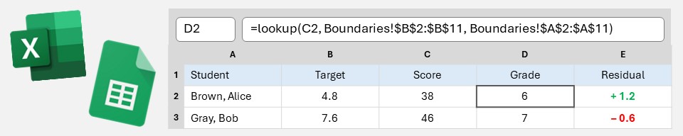
In cell E4, we’re now going to enter a formula instead of a grade:

=LOOKUP(D4,Boundaries!$B$2:$B$11,Boundaries!$A$2:$A$11)

The LOOKUP function finds the first argument (whatever is in cell D4, ie the score) within the second argument (the boundaries for Test 1 on the Boundaries sheet) and returns whatever is in the corresponding row of the third argument (the grades on the Boundaries sheet).

We’re now going to copy this formula down the entire column: double click the highlighted little black square (or left-click it and drag it downwards). When we do this, the spreadsheet will automatically update the reference to D4 (changing it to D5, D6, D7, etc), but we don’t want it to do this to the references on the Boundaries sheet. This is what the $ signs achieve; by writing $B$2 instead of B2, it fixes the range so that is doesn’t change when we copy the formula to other cells.

Note: LOOKUP is an old function that has received a couple of upgrades over the years, first to VLOOKUP and then more recently to XLOOKUP. The newer functions are cleverer, more versatile and faster…however, for what we’re doing above you are not going to notice the difference and LOOKUP is easier to implement! Just understand that the second argument (the boundaries) must be sorted in ascending order otherwise LOOKUP will give the wrong result. If, for whatever reason, your scores are not sorted in ascending order, you will need to use XLOOKUP instead:

=XLOOKUP(D4,Boundaries!$B$2:$B$11,Boundaries!$A$2:$A$11,,-1)

They’re the same except for the “,,-1” at the end. The “-1” requests an approximate match rather than an exact match, in this case the highest match lower than or equal to the score. (LOOKUP naturally defaults to this approximate match.)

Compare the grade to the target

In cell F4, we’re going to add in a simple comparison to the target: =E4-C4. Again, we’ll copy this down the entire column.

(If the grades are letters instead of numbers, we’ll need to a conversion first — see “A Level grades”, below.)

To make this residual easier to interpret, we’re going to apply some formatting to it.

First, we’ll force a “+” sign to accompany positive values. In Microsoft Excel, press <CTRL><1> (or Home > Number > Format > Custom). In Google Sheets, select Format > Number > Custom Number Format. In the box that appears, type + 0.0; - 0.0; This puts a + on positive numbers, a – on negative numbers, hides zero values and insists on 1 decimal place.

Second, we’re going to add some conditional formatting to change the colour.

In Excel, Home > Conditional Formatting > New Rule. Choose “Format only cells that contain” and choose “Greater than” and zero. Change the font formatting to bold green. Repeat for “Less than” and bold red.

In Sheets, you need to select Format > Conditional Formatting and then do as above:

Once more, copy F4 down the column (or use the format painter tool) to copy to the other cells. The final result is:

Finishing touches: Error traps

The two columns that we’ve added formulae to will only work properly once a score has been entered. Until then, we unhelpfully get this:

To prevent this, we need an upgraded version of of our formulae, to include some error traps:

=IF(ISNUMBER(D4),LOOKUP(D4,Boundaries!$B$2:$B$11,Boundaries!$A$2:$A$11),"")

=IF(AND(ISNUMBER(C4),ISNUMBER(E4)),E4-C4,"")

Here, the IF function checks if there is a number in the score column (and the target column, for the residual). If there is, it carries out our formula, but if not it leaves the cell empty.

Finishing touches: Generate a group or cohort residual

More usefully than having a “+/-” column header is displaying the average residual for the displayed students.

This is achieved by entering the following formula in the cell instead of “+/-“:

=IFERROR(SUBTOTAL(1,$G$4:$G$503),"")

The SUBTOTAL function has lots of uses, but the “1” argument makes it calculate the average of the displayed values. This means that if we add a column for teaching group and turn on filters, when we filter to a particular group the average will only be for that group.

The use of “503” is just to ensure that the average reaches down the sheet far enough. This allows for 500 students in your cohort. If you have more, increase this number.

The IFERROR function wrapping the SUBTOTAL function is another error trap — it will display an empty cell if there are no scores yet.

A Level grades

When calculating the residual above, we assumed that the grades and targets were GCSE-style numbers. However, what if they are A Level-style letters, A* to E? In this case, we’re going to need to add a conversion table to our Boundaries sheet, so that we can turn our letters into numbers. For example:

We can now look up a numerical score from the grade. Due to this table not being sorted in ascending order, we’re going to use XLOOKUP rather than LOOKUP:

XLOOKUP(F4,Boundaries!$K$2:$K$8,Boundaries!$L$2:$L$8)

This looks a lot like our LOOKUP formula, but this one doesn’t mind the sort order and also only returns exact matches, whereas our previous formula returned the largest match below or equal to our score (ie an approximate match).

We need to put this where “F4” was in our previous residual formula of =F4-D4:

=XLOOKUP(F4,Boundaries!$K$2:$K$8,Boundaries!$L$2:$L$8)-D4

If the target in D4 is also a letter rather than a score, the “D4” will need replacing with the (same) XLOOKUP formula, too.

With whole-number targets like above, you will probably also like to modify the custom number format of the residuals to lose the decimal place: + 0; - 0; .

Impact on efficiency

In terms of working smarter and saving you time, what the above does is quickly highlight to you the students who need positive recognition and those who need some form of intervention. Filtering the residual column to “+0.5 and above” or “-0.5 and below” does this for you in moments. You become more effective as a teacher and the bonus is that it takes no time to do so!